Time Series Analysis with Components

Click to learn more about co-author Maarit Widmann.

Click to learn more about co-author Daniele Tonini.

Click to learn more about co-author Corey Weisinger.

Time Series Forecasting is often neglected says Professor Daniele Tonini:

“Considering the plethora of articles, applications, web tutorials and challenges on the data science subject that we’re seeing in the last 3-5 years, it can be pretty surprising to find only a few of them dedicated to time series analysis and forecasting. We’re living in the golden era of data analytics, with plenty of data and algorithms of any kind… but topics like deep learning, artificial intelligence and NLP are attracting basically all of the attention of the practitioners, while the concept of Time Series Forecasting is often neglected. Since many forecasting methods date back decades, it’s quite easy to say “nothing particularly interesting there… Let’s focus on that brand-new machine learning algorithm!”

But this could be a great mistake, since more accurate and less biased forecasts can be one of the most effective drivers of performance in business, operations, finance and science (and by the way, to be clear, the innovation in Time Series Analysis is nowadays still animated, if you dig deeper under the surface). Knowing the basics of Time Series Analysis is one essential step in the Data Science world that enables important capabilities in dealing with sequence and temporal dynamics, in order to move beyond the typical cross-sectional data analysis. Facing the fundamentals of forecasting with time series data, focusing on important concepts like seasonality, autocorrelation, stationarity, etc is a key part of this type of analysis.

Forecasting can feel like, and in many ways truly is, a completely different beast than other data science problems such as classification or numeric prediction. It fits into a different paradigm than the traditional “data in; prediction out” of the prior cases.

In conjunction with Professor Daniele Tonini of the University of Bocconi in Milan Italy we’ve built a set of components in KNIME to help get started on this task. A component is a node that encapsulates the functionality of a workflow, such as training an ARIMA model. Components can be reused and shared locally, via the Server, or on the Hub.

The components for time series analysis cover various tasks from aggregating and inspecting seasonality in time series to building an AutoRegressive Integrated Moving Average (ARIMA) model and checking the model residuals. These components use the Python integration, extending the analytical capabilities of KNIME Analytics Platform for time series analysis with the statsmodels module in Python. However, the code only executes in the background, and you can define the settings for each task, as for any other KNIME node: in the component’s configuration dialog.

The time series components are available on the Hub. Drag and drop them into your workflow editor and start building your workflows for time series analysis!

*Figure 1: Accessing a time series component: drag and drop the component into your workflow edito*r

In this blog post we want to take a moment to introduce just a few of these new components and talk about how they slot together into a Time Series Analysis pipeline.

Steps in Time Series Analysis

Let’s say you have a sensor attached to something, maybe the electrical meter on your house, and you want to plan your budget. You need to forecast how much power you’ll use in the future.

Time Aggregation

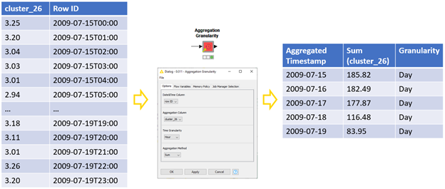
The first step we might take after accessing this sensor data is to reduce it into a manageable shape. Aggregating this data, perhaps to the hour, will not only reduce the data size substantially, but also smooth out some of the noise.

For this operation, we’ll need the Aggregation Granularity component that generates daily total energy consumption from hourly data. Many granularities and aggregation methods are available, and we could also generate, for example, monthly average values from daily data. (Figure 2):

Figure 2: Aggregating time series by selected granularity and aggregation method using the Aggregation Granularity component. In this example we calculate daily total values of the “cluster_26” column.

Timestamp Alignment

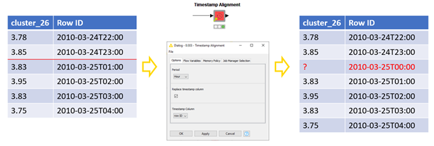
Next we need to verify our data is clean. One assumption time series models require is continuously spaced data. But what if our sensor was busted or we used no power for an hour?

If we find gaps in our time series, we fill them in. We just need to define the granularity of the spacing, which determines a gap as a missing minute, hour, or day, for example. The inserted timestamps will be populated with missing values that can be replaced by, for example, linear interpolation of the time series. (Figure 3):

Figure 3: Filling gaps in time series using the Timestamp Alignment component. In this example, the energy consumption for the last hour on March 24, 2010 is not reported. Therefore, the timestamp is added to the time series and populated with a missing value.

Inspecting Seasonality and Trend

Ok, so we’ve got aggregated, cleaned data. Before we get into modeling it’s always good to explore it visually. Many popular models assume a stationary time series, this means, its statistics remain the same over time. Therefore, we decompose the time series into its trend and seasonalities and finally fit the model into its irregular part.

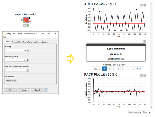
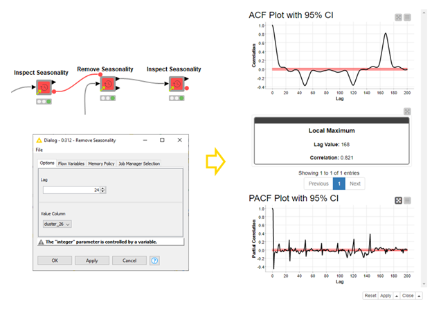
We can inspect seasonality in time series in an autocorrelation (ACF) plot. Regular peaks and lows in the plot tell about seasonality in the time series, which can be removed by differencing the data at the lag with the greatest correlation. To find this local maximum, we use the Inspect Seasonality component (Figure 4). To remove the seasonality at the local maximum, we use the Remove Seasonality component. The second, third, etc. seasonalities can be removed by repeating this procedure. (Figure 5):

*Figure 4: Inspecting seasonality in time series using the Inspect Seasonality component. The highest correlation is found between the current value and the value 24 hours before.*

Figure 5: Removing seasonality in time series using the Remove Seasonality component. In this example, the first (daily) seasonality is removed by differencing the data at the lag 24, which is the first (daily) seasonality given by the Inspect Seasonality component. The autocorrelation plot shows now the second (weekly) seasonality, which can be removed using the Remove Seasonality component another time.

Automatically Decomposing a Signal

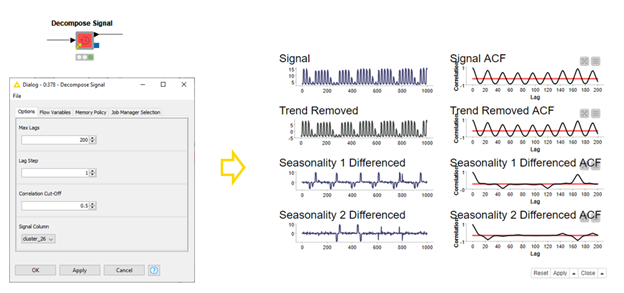
In the previous section we inspected our signal and differenced it. Then we inspected the second seasonality and differenced it. This is a perfectly good strategy and gives you complete control over the processing of your data. We’ve also published a component called Decompose Signal. It will automatically check your signal for trend, and two levels of seasonality; returning the decomposed elements and the residual of your signal for further analysis (Figure 6). Perhaps with our ARIMA components in the next section?

Figure 6: The output view of the Decompose Signal component. The view shows the progress of the Signal as it progresses through the decomposition stages as well as the respective ACF Plots. In this example, we remove a (very minor) trend, and two layers of seasonality shown in the line plots on the left. The two first seasonalities are daily (24) and weekly (168).

Building ARIMA Models

We’re nearly there now, we’ve satisfied the stationarity requirement of models like the ARIMA. We can build this model easily with the new (Auto) ARIMA Learner components.

When we build an ARIMA model, we need to define three parameters that define which temporal structures are captured by the model. These parameters tell the relationship between the current value and the lagged values (AR order), between the current forecast error and the lagged forecast errors (MA order), and the degree of differencing required to make the time series stationary (I order). The best AR, I, and MA orders can be defined by exploring the (partial) autocorrelation plots of the time series.

With the AR, I, and MA orders defined, we can then train the ARIMA model. However, defining the parameter values is not always straightforward. In such a case, we can give the maximum values for these parameters, train multiple ARIMA models, and select the best performing one based on an information criterion AIC or BIC. We can do this with the Auto ARIMA Learner component. Both components output the models, their summary statistics and in-sample forecasting residuals. (Figure 7):

Figure 7: Training an ARIMA model using the ARIMA Learner and Auto ARIMA Learner components. The ARIMA Learner component trains a model with pre-defined AR, I, and MA orders. The Auto ARIMA Learner component trains multiple models with different combinations of the AR, I, and MA orders within the defined range, and produces the best performing model in its output. The data outputs of the components show the model summary statistics and in-sample forecasting residuals.

Forecasting by ARIMA Models

Finally we’re ready to model, we need to generate that forecast so we can fill in the energy line item on our budget!

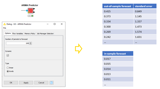
The ARIMA Predictor component applies the model to the training data and produces both in-sample and out-of-sample forecasts. For the out-of-sample forecasts we need to define the forecast horizon. In our case here, we select a forecast horizon “1” if we’re interested in the estimated energy consumption in the next hour, 24 for the next day, 168 for the next week, and so on. For the in-sample forecasts we can either use the forecast values to generate new in-sample forecasts (dynamic prediction), or use the actual values for all in-sample forecasts. In addition, if the I order of the ARIMA model is greater than zero, we define whether we forecast the original (levels), or differenced (linear) time series. (Figure 8):

Figure 8: Producing in-sample and out-of-sample forecasts with the ARIMA Predictor component. We can control firstly the number of out-of-sample forecasts, secondly whether actual or forecast values (dynamic prediction) are used for in-sample forecasting, and thirdly whether the original or differenced time series is forecast, if the model’s I order is greater than zero.

Analyze Forecast Residuals

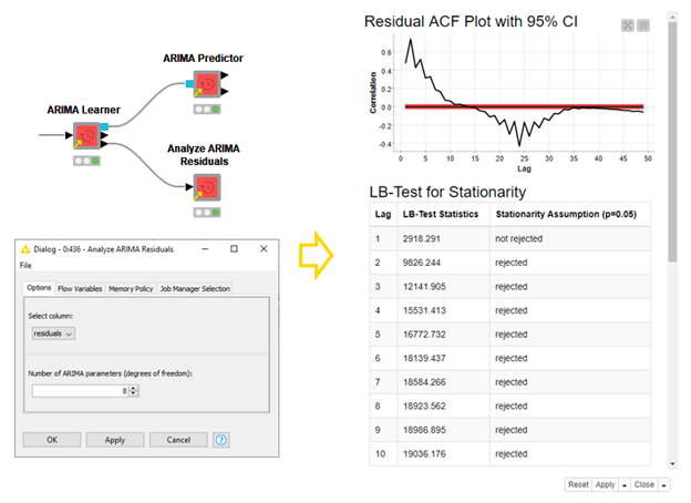
Before we deploy our model and really take advantage of it, it’s important we are confident in it. KNIME analytics platform has many tools for analyzing model quality, from ROC curves to confusions matrices with the scorer nodes to statistical scores like MSE. We’ve also added a component specifically built for ARIMA residuals: The Analyze ARIMA Residuals component. This component will apply the Ljung-Box test of autocorrelation for the first 10 lags and report if the stationarity assumption is rejected, or not, based on a 95% confidence level (Figure 9). It will also show the ACF Plot for the residuals, and a few other diagnostic plots.

Figure 9: Output view of the Analyze ARIMA Residuals component that shows the ACF Plot as well as the LB-Test statistics, and if you scroll further down the residual time plot and normality measures. To use the Analyze ARIMA Residuals component simply select the residual data column and the proper degrees of freedom for your input model.

Summing up!

In this blog post, we have introduced a few steps in time series analysis and how to perform the different operations from preprocessing to visualizing, decomposing, modeling, and forecasting time series using the time series components available on the Hub.

Of course, the required operations in preprocessing time series are often more than just aggregating time series and inspecting seasonality. Besides ARIMA models, time series can also be forecast using classical methods, machine learning based methods, and neural networks.

LEARN MORE ABOUT OUR ENTERPRISE TRAINING BUNDLES

Data Topics