Click to learn more about author Thomas Frisendal.

Timely Concerns in Data Models

In June I published a blog post called Timely Concerns in Data Models. In summary the concerns that I mentioned in June were: Roles of time (such as Valid Time, Recorded Time, As-Is vs. As-Of, Read timelines, Time Series), The scope of the time vs. the functional dependencies and agile schema evolution. I followed this up in July with The History of Time in Data Models.

I promised to get back to you on these issues. So, here we go: Join me in this quest for defining (parts of) the future history of temporal data modeling! Let’s start with SQL.

Are the Basic Time Concepts in Standard SQL not Enough?

I think that maybe not all readers are familiar with the actual features of temporal SQL, so here follows a brief overview, based on a SQL Technical Report — Part 2: SQL Support for Time-Related Information (SQL:2015 standard) from ISO, the International Standards Organization (www.iso.org).

Basically, there are three predefined datetime datatypes:

• TIMESTAMP (having YEAR, MONTH, DAY, HOUR, MINUTE and SECOND
• DATE (having YEAR, MONTH, and DAY
• TIME (having HOUR, MINUTE and SECOND)

SECOND may be specified with a defined number of digits of fractional seconds. TIMESTAMP and TIME may be specified “… WITH TIME ZONE”.

The same ISO technical report also describes the semantics of INTERVAL(s), which may be either on the Year/Month level or on the Day/Hour/Minute/Second level.

SQL tables may be associated with PERIOD(s). Such as here: “…. PERIOD FOR business_time (bus_start, bus_end)”, where bus_start and bus_end are columns of the table.

Predicates, which may be applied to PERIOD(s) are OVERLAPS, EQUALS, CONTAINS, PRECEDES and SUCCEEDS. The last two may be supplemented with IMMEDIATELY.

Application Periods for SQL Tables

The SQL implementation should be able to handle application (business data content) level versioning (valid from / valid to) using extensions such as:

“… PRIMARY KEY (emp_id, business_time WITHOUT OVERLAPS),

FOREIGN KEY (dept_id, PERIOD business_time) REFERENCES

dept (dept_id, PERIOD business_time)”

System-versioned SQL Tables

The SQL implementation should also be able to handle database update level versioning (recorded from / recorded to) using extensions such as:

“CREATE TABLE Emp (ENo INTEGER, Sys_start TIMESTAMP(12) GENERATED ALWAYS AS ROW START, Sys_end TIMESTAMP(12) GENERATED ALWAYS AS ROW END, EName VARCHAR(30), PERIOD FOR SYSTEM_TIME (Sys_start, Sys_end)

) WITH SYSTEM VERSIONING”

SQL and Temporal Support

Together, application periods and system versioning is a scheme for doing basic bitemporal data modeling.

An “as-of” query looking for recorded information in a given period of time can look like this:

SELECT ENo,EName, Sys_Start, Sys_End

FROM Emp FOR SYSTEM_TIME

FROM TIMESTAMP ‘2011-01-02 00:00:00’ TO TIMESTAMP ‘2011-12-31 00:00:00’

However, the interval obviously applies to each and every column of the table under version control. But it is clear that:

Consequence no. 1: Given that the SQL standard is so widely used, temporal SQL is part of the picture.

Furthermore, I do believe that the two “predefined” kinds of timelines (application and system) are too few. We need more flexibility. As you can see from the list of concerns above, there are a handful more, perfectly reasonable, roles of timelines to support. No. 3 on my list would be a schema changes timeline.

Richer Time Ontologies

OWL-Time from the W3C

The World Wide Web community (W3C) has defined the OWL-RDF stack used in the web and in linked open data. Part of the ontology offerings is the OWL-Time ontology.

OWL-Time is a good ontology that covers most aspects of time and (one-dimensional) temporality. The diagram below shows some key parts of it:

OWL-Time is a good ontology that covers most aspects of time and (one-dimensional) temporality. The diagram below shows some key parts of it:

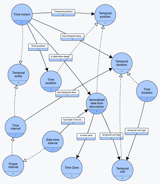
(The diagram is drawn from the W3C OWL source using gra.fo, which is a commercial graph modeling tool from data.world).

OWL-Timeline

Built on top of OWL-Time, the OWL-Timeline ontology has some nice additional qualities. It opens up for multiple timelines of multiple types (relative, physical, continuous, and discrete) and also supports mapping between timelines.  Here is another (gra.fo) diagram of selected parts of the ontology:

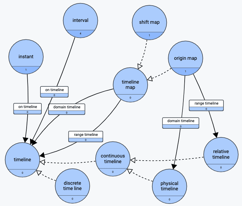
This OWL ontology is authored by Yves Raimond and Samer Abdallah (of Centre for Digital Music at the Queen Mary University in London), and it is part of the Music Ontology project at the university. It is being used in several, large production sites at the BBC, MusicBrainz and the Musicweb et al.

Consequence no. 2: This kind of conceptual thinking certainly offers richer features needed in  the future of temporal data modeling.

The other issue is tables as temporal target versus more detailed versioning.

Which Data Models, by the Way?

Is it Game Over for Tables?

Now that we know that we have some standards (SQL and OWL), at hand, which can boost the temporal modeling space, we need to think about the scope of the temporality. What is the “atom” of temporality? The answer lies in the dependencies.

Much (if not all) of the discussion about temporal issues in the last 30+ years have been based on the assumption of the necessity of SQL tables. The narrative for how to build “well-formed” SQL data models is the well-known “Normalization” procedure. Data modelers with my hair color will remember the poster, which was a give-away with the Database Programming and Design Magazine (Miller Freeman) in 1989. The title of the poster is “5 Rules of Data Normalization”. Here is a miniature image of it:

You can see a readable version of the poster at this site. The intellectual rights belong to Marc Rettig (now at Fit Associates, Design for Social Innovation and CMU School of Design). Thanks to Marc for still sharing this collector’s item! The narrative is about modeling a database containing data about puppies and kennels. 🐕 🐕 🐕 😃

In retelling the narrative, I will be using my own visual normalization technique, which I developed in my 2016 book Graph Data Modeling for NoSQL and SQL.

So, Bella, (good dog), here we come!

From Chaos to Consistence in 3 Easy Steps

Here is a list of the data, we want:

Puppy Number, Puppy Name, Kennel Code, Kennel Name, Kennel Location,

Trick ID 1..n, Trick Name 1..n, Trick Where Learned 1..n, Skill Level 1..n

The first 3 steps are rather easy. (I loyally follow the poster).

1. First, we should eliminate repeating groups. That will give us two tables, one containing the first 5 fields and the other containing the last 4 fields (which is a repeating group).

• Next, we should remove redundant data. Well, Trick Names would be repeated redundantly, so we need to split the second table, we just made, into two: One for the Tricks as such, and one for the Tricks, which each puppy masters.

• The third thing is to split according to keys. Clearly, the first table we just made, is a mix of two sets of data: One for the Puppies and one for the Kennels.

In this manner we arrive at a model, which is consistent with respect to cardinalities, redundance and identities. But, IMHO, it is much easier to draw it as a graph right from the start and ponder about the 3 rules, as you whiteboard the graph:

As it happens, we learn by observation that there are two kinds of dependencies behind the scenes:

• Intra-table dependencies, which is the classic functional dependency of properties, which “hang off” the key of some object (type) identified by that key (color of a product, for example) , and
• Inter-table dependencies, where some object (type) is “pointing” to the key of another object (type), such as an employee working in a department, the relationships, really.

The classic normalization narrative did not bother about naming the dependencies. Names of dependencies contain clues about the nature of them. If the name contains active verbs, like “Puppy can do Puppy Trick”, it is probably a relationship, whereas a passive verb, like “Puppy has Puppy Name” denotes a property of an object.

If you whiteboard these things, most of the structure comes by itself.

Identity and uniqueness are also easy by way of visualization. Clearly the uniqueness of Puppy Trick is the combination of the uniqueness keys of Trick (Trick Id) and Puppy (Puppy Number). So maybe a good idea would be to introduce a Puppy Trick Id (system generated) to easily establish the identity of a Puppy Trick. The visuals (not least the dependencies) tell the full story.

“Semantic Consistence”

Having established identity consistence (3 NF), we are ready to look for more subtle structures. (Note: I am still loyally following the poster example’s two last steps).

4NF: We are asked to introduce a new piece of data, namely a Costume that the Puppy can wear. As you can see below, it is visually rather easy to see that the Costume is a separate thing belonging to a Puppy (and, ideally, also a Costume type). Formally, we have isolated two independent relationships, 4NF.

5NF: The last step in the poster example is a rather complex set of business rules, when it comes to marshalling out the structure, because they involve 3 relationships, which go together to support the rules. Again, the graph visualization is a great help. (Refer to the poster for the details). Formally, we have isolated independent multiple relationships, 5NF.

The Semantic Consistence state can also be visualized as a property graph, like this:

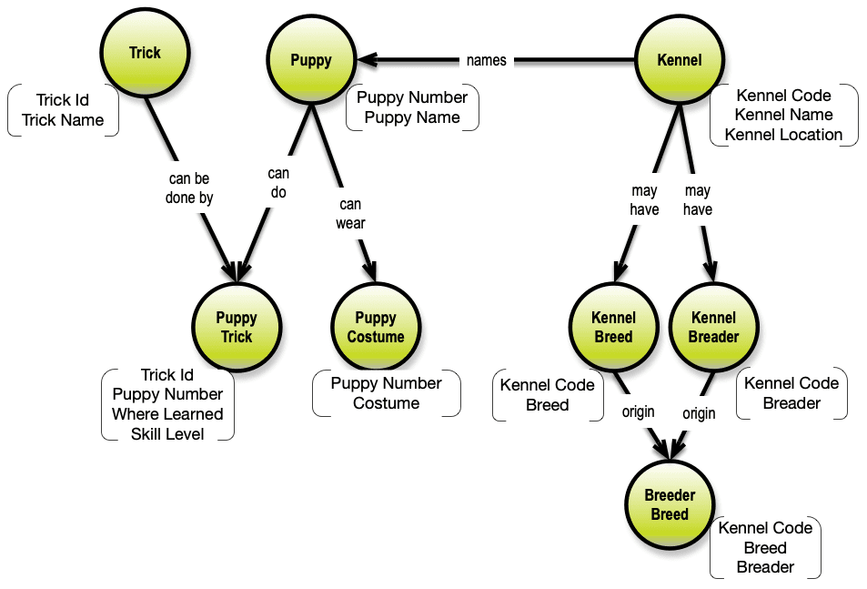
Note that this is 5NF and it could also be mapped easily to a data vault model in SQL tables. So, if you used this model as the basis of the temporal extensions, you could do that, but you would have to version e.g. the 3 values of Kennel Code, Kennel Name and Kennel Location using the same timeline periods (intervals). Or you will have to decompose the model further.

Complete Consistence for Temporal Extensions

Bundling together properties because they go together in 5NF is too coarse. That is why the concept model, which we arrived at under semantic consistence is actually the most completely consistent model of them all:

This is also known as 6NF. Maps easily to an Anchor Model, by the way.

Consequence no. 3: The table paradigm is too coarse for precise and complete temporal support. We need a graph representation going down to the atomic concept level (6 NF) for doing that

The advantages of doing temporal extensions on this, the lowest, level are:

• Each and every attribute can be associated with as many timelines as necessary
• The same goes for both dependencies (properties of node types) as well as relationships (start- and end-nodes etc.).
• The complete consistence level is close to the physical primitives that many graph databases are using behind the curtains.

You may also apply temporality one up level at the 5NF representation (or maybe even 3NF) and apply temporal extensions there (at the node/label level for property graphs or the table level for SQL tables).

What matters is complete understanding of the semantic graph linking all concepts and their dependencies.

OK – Where Should We Declare the Temporal Extensions?

In the Schema, of course. But that is a naïve answer.

For SQL, the answer is: Yes, Schema / DDL commands. And SQL is engaged to adopt a property graph extension, for read-only purposes to begin with. Once that is in place (probably in 2020), the SQL data definition syntax is a factor to consider.

For non-SQL property graphs the picture is blurred. Some DBMS’s have more schema functionality than others. There currently is no standard for property graph schemas. But people are working it. The ambition is to have something (a phase one) also in 2020. The first version will probably not support temporal extensions.

The proposed new standard language has the working title GQL. The work is carried out both in the ISO organization (ISO/IEC JTC 1/SC 32/WG 3) as well as in community-based groups (soon to become task forces in of the LDBC Council).

So, the answer to where to define the timelines, really is: Eventually in the schema(s), once property graph schemas are ready. This gives vendors some time to consider (and I have some ideas I would like to contribute).

The result could be a temporal landscape somewhat like the following.

Kinds of Timeline and Temporal Declarations 

Data (Content) Changes

The conceptual structure for applying timelines to data content is rather simple. The only value-carrying parts are the properties:

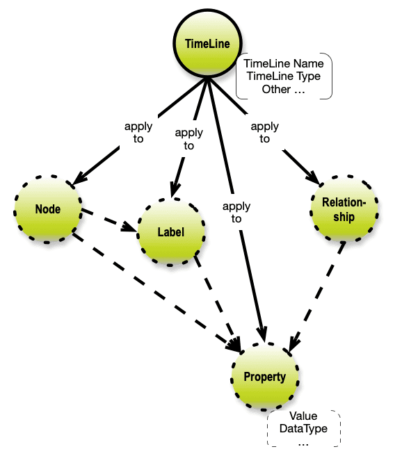
Timelines should also be applicable on the Node, Label and Relationship levels. Implying that a timeline applies to all properties owned directly or indirectly from that node / label / relationship.

One of the timelines is the “system-versioned” variety (to comply with SQL).

The application period timelines need to be anchored in both a begin- and an end-instant, which stick to the data item, which is controlled by the timeline. (A property, a node label, a relationship etc.).

If the property graph is a 5NF (or maybe even 3NF) instance, the above applies as well, but begin/end applies to all properties on the level. The DBMS engine must still understand the full complete (6NF) graph structure in all cases.

Schema Change Timelines

For schema changes the picture is, obviously, somewhat more complex.

Most of the property graphs data model’s constituent parts may change. Names (incl. Labels), of course, and datatypes of properties. But as important are the structural changes (add / delete) as well as change. A property, for example may move from one label to another or a relationship may change direction, from- or to- node types (Labels) etc. Relationships may, unless they are restricted be many-to-many. There are some interesting challenges here.

Remember that property graphs are frequently developed iteratively and several data products are of the schema last type. But the direction many people are going is a full schema, eventually.

As for timeline types on the schema side, I figure the “system-versioned” type will be quite popular.

Timeline Mappings

This topic is also interesting, not least to establish ways of consolidating temporal information across different timelines and timeline types.

The goal must be to make the necessary definitions short and precise, thus enabling users to, using simple queries, ask temporal questions (moving the efforts away from the data modelers over onto the DBMS systems).

Query Considerations

The full, explicit, multi-dimensionality of timeline networks within graphs is actually a bit frightening. Here is an example of just a little snippet of a graph with just three timelines applied:

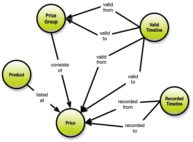
On the query level, there should be as little to do as necessary to include predicates in the selection criteria. It could be as simple as:

“… VALIDITY WITHIN (TIMESTAMP ‘2019-01-02 00:00:00’ TO TIMESTAMP ‘2019-03-31 00:00:00’) AND RECORDED WITHIN (TIMESTAMP ‘2019-02-01 00:00:00’ TO TIMESTAMP ‘2019-02-07 00:00:00’) …”

The full specter of predicates listed in the section about ontologies should be applicable. But the interval logic should go on behind the scenes. An additional “ORDER BY <timeline>” would come in handy.

Consequences for the Future History of Temporal Modeling

As a conclusion, the following is what I (would like to) see happening in the future of temporal data modeling.

1. The ISO SC32 (SQL standard) committee has an important job to do, and I believe they will deliver on target in 2020. That means that we will have property graph support in SQL, and that there will (maybe somewhat later) be a standard property graph schema language (and a query language as well).
2. Work must start soon, in order for the extended timeline ontologies to meet and match the SQL functionality, thus influencing the way the consorted effort towards a new property graph standard (that interoperates with SQL) will look like. Whether this will happen on the standards train or initially by first-moving vendors is uncertain. I could suspect the latter. (Solid temporal support will sell well on Wall Street).
3. The requirements for timelines in temporal data modeling is stressing the current solution architecture on top of SQL, so the bar needs to be raised. I think the two OWL ontologies is a good source of inspiration for building a broader conceptual paradigm for flexible, dynamic temporal timelines.

Once somebody has developed the above (and it is doable), we have achieved what should be called “True Full Scale Data Modeling”.

The business cases are many, spanning from government over finance, compliance, complex systems, life at risk applications etc. And I am sure that the schema change timeline type will deliver on some serious business requirements. 3 timeline configurations across multiple properties can be easy to define, and to work with. But you need to deal with them on the 6NF level.

The Future Starts NOW!

As we have seen, temporal dependencies quickly explode into a highly connected network, which  best can be handled by a graph DBMS.

It also follows that the complexity must be hidden for both data modelers and business users by way of some higher-level concepts, as I have sketched out in this post.

Admitted, I wrote this post to provoke vendors into considering this architectural sketch for their future product development. We are talking about much needed features of commercial DBMS products.

Dear implementers, it is about time!