In this blog post, I’d like to introduce some basic concepts of reinforcement learning, some important terminology, and a simple use case where I create a game playing AI in my company’s analytics platform. After reading this, I hope you’ll have a better understanding of the usefulness of reinforcement learning, as well as some key vocabulary to facilitate learning more.

Reinforcement Learning and How It’s Used

You may have heard of reinforcement learning (RL) being used to train robots to walk or gently pick up objects; or perhaps you may have heard of Deep Mind’s AlphaGo Zero AI, which is considered by some to be the best Go “player” in the world. Or perhaps you haven’t heard of any of that. So, we’ll start from the beginning.

Reinforcement learning is an area of machine learning and has become a broad field of study with many different algorithmic frameworks. In summary, it is the attempt to build an agent that is capable of interpreting its environment and taking an action to maximize its reward. 

At first glance, this sounds similar to supervised learning, where you seek to maximize a reward or minimize a loss as well. The key difference is that those rewards or losses are not obtained from labeled data points but from direct interaction with an environment, be it reality or simulation. This agent can be composed of a machine learning model – either entirely, partially, or not at all. 

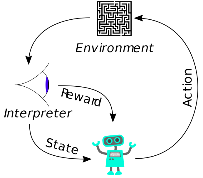
A simple example of an agent that contains no machine learning model is a dictionary or a look-up table. Imagine you’re playing “Rock-Paper-Scissors” against an agent that can see your hand before it makes its move. It’s fairly straightforward to build this look-up table, as there are only three possible game states for the agent to encounter.

This can get out of hand very quickly, however. Even a very simple game such as Tic-Tac-Toe has nearly 10 million possible board states. A simple look-up table would never be practical, and let’s not even talk about the number of board states in games like Chess or Go.

This Is Where Machine Learning Comes into the Equation

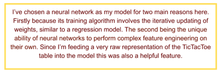
Through different modeling techniques, commonly neural networks – thanks to their iterative training algorithm – an agent can learn to make decisions based on environment states it has never seen before.

While it is true that Tic-Tac-Toe has many possible board states and a look-up table is impractical, it would still be possible to build an optimal agent with a few simple IF statements. I use the Tic-Tac-Toe example anyway, because of its simple environment and well-known rules.

Real-World Applications of Reinforcement Learning

When talking about reinforcement learning, the first question is usually “What’s that good for?” The examples above are very far removed from most practical use cases; however, I do want to highlight a few real-world applications in the hopes of inspiring your imagination.

• Chemical Drug Discovery: Reinforcement Learning is often used to create chemical formulas/compounds with a desired set of physical properties, according to the following sequence of actions: Generate compound > test properties > update model > repeat.
• Bayesian Optimization: Included in the Parameter Optimization Loop, this strategy iteratively explores the parameter space and updates a distribution function to make future selection decisions. 
• Traffic Light Control: Reinforcement learning has made huge strides here as well. However, in this case, the partially observable nature of real-world traffic adds some layers of complexity. 
• Robotics: This is likely the most famous of these use cases. In particular, we’ve seen many examples of robots learning to walk, pick up objects, or shake hands in recent years.

Even if none of these use cases hits close to home for you, it’s always important that a data scientist continually adds new tools to his belt, and hopefully, it’s an interesting topic besides. 

Adding Formality

Let’s now lay out a more concise framework.

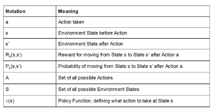
Basic reinforcement learning is described as a Markov Decision Process. This is a stochastic system where the probability of different outcomes is based on a chosen Action, a, and the current Environment State, s. Specifically, this outcome is a New Environment State that we’ll denote s’. 

Let’s define two functions on top of these terms as well: R_a(s,s’) and P_a(s,s’). R_a(s,s’) denotes the reward assigned when moving from state s to state s’, and _Pa(s,s’) the probability of moving from state s to s’, given action a.

So, we’ve defined the system, but we’re still missing one part. How do we choose the Action we should take at State s? This is determined by something called a Policy Function denoted as ℼ(s). Some simple examples of a Policy Function might be:

• ℼ(s) = move up
  • when navigating a grid
• ℼ(s) = hit me
  • when playing blackjack
• ℼ(s) = a; where a is a random element of A
  • when using a machine learning model for ℼ(s) we may start from this point to gain a varied data set for future trainings

A Policy Function could be much more complicated as well. Such as a huge set of nested IF statements … but let’s not go there.

What We’ve Done So Far 

1. Determine action to take at the current State s

• a = ℼ(s)

2. Determine New State s’

• This new state is often stochastic, based on P_a(s,s’)

3. Determine the Reward to be assigned to action a

• Reward is based on some function R_a(s,s’) depending on the chosen action a. For example, there is some intrinsic reward if I get to work in the morning, but far less if I chose to charter a helicopter to take me there … 

Choosing a Policy Function

Let’s talk more about the Policy Function ℼ(s). There is a myriad of options for ℼ(s), when using machine learning, but for the sake of this article, I want to introduce one simple example: An agent I’ve built to play Tic-Tac-Toe.

I mentioned above that for Tic-Tac-Toe, there are far too many board states to allow for a look-up table. However, at any given State, s, there are never more than nine possible Actions, a. We’ll denote more concisely these possible actions at state s as A_s, contained in A. If we knew what the reward would be for each of these possible actions, we could define our Policy Function to produce the action with the highest reward, that is:

ℼ(s) = a | Max_a∈As R_a(s, s’)

Reward Function

Among the many possible reward functions, we can choose to quantify how close to winning – or losing – the move brought the Agent. Something like:

R_a(s,s’) = 0.5 + [# of Moves played so far] / 2*[# of Moves in game] if Agent wins

0.5 – [# of Moves played so far] / 2*[# of Moves in game] if Agent loses

However, this reward function is undetermined until the game is over and the winner becomes known. This is where we can apply machine learning: We can train a predictive model to estimate our reward function, implicitly predicting how close this move will take the agent to win. In particular, we can train a neural network to predict the reward given some action. Let’s denote this as:

NN(a) ~ R_a(s,s’)

Neural Network Training – Supervised Learning

At this point, the problem has moved to the training of a neural network, which is a supervised learning problem. For that, we need a training set of labeled data, which we can collect by simply letting our network play the game. After every game has been played, we score all the actions, through the original Reward Function R_a(s,s’). On these scores on the actions in all played games, we then train a neural network to predict the reward value – NN(a) – for each action in the middle of the game.

The network is trained multiple times on a new training set including the latest labeled games and actions. Now, it does take a lot of data to effectively train a neural network, or at least more than we’d get from just one or two games. So how can we collect enough data? 

As a final theoretical hurdle, it should be noted that neural networks are, typically, deterministic models and, if left to their own devices, will always make the same predictions given the same inputs. So, if we leave the agent to play against itself, we might get a series of identical games. This is bad, because we want a diverse set of data for training. Our model won’t learn much, if it always plays the exact same game move after move. We need to force the network to “explore” more of the move space. There are certainly many ways to accomplish this, and one is to alter the policy function at training time. Now instead of being:

ℼ(s) = a | Max_a∈As NN(a)

It becomes the following, which enables the agent to explore and learn:

ℼ(s) = a | Max_a∈As NN(a) with probability 0.5

= a ∈ A_s with probability 0.5

A common approach is to alter the above probabilities dynamically, typically decreasing them over time. For simplicity I’ve left this as a constant 50/50 split.

Implementation

Now for the implementation! We need to build two applications: one to train the agent and one to play against the agent.

Let’s start with building the first application, the one that collects the data from user-agent games as well as from agent-agent games, labels them by calculating the score for each action, and uses them to train the neural network to model the reward functions. That is, we need an application that:

• Defines the neural network architecture
• Implements the reward function R_a(s,s’), as defined in the previous section, to score the actions
• Implements the latest adopted policy function ℼ(s)
• Lets the agent play against a user and saves the actions and result of the game
• Lets the agent play against itself and saves the actions and result of the game
• Scores the actions
• Trains the network

For the implementation of this application we used my company’s analytics platform, because it is based on a Graphical User Interface (GUI) and it is easy to use. The platform extends its user-friendly GUI also to the Deep Learning Keras integration. Keras libraries are available as nodes and can be implemented with a simple drag and drop.

The Network Architecture

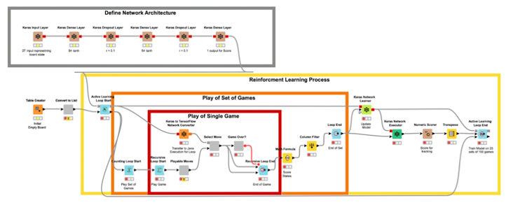
In the workflow in Fig. 5, the brown nodes, the Keras nodes, at the very top build the neural network architecture, layer after layer. 

• The input layer receives a tensor of shape [27] as input, where 27 is the size of the board state. The current state of the board is embedded as a one-hot vector of size 27.
• The output layer produces a tensor of shape [1] as the reward value for the current action. 
• The middle 2 hidden layers, with 54 units each, build the fully connected feedforward network used for this task. These 2 layers have a dropout function, with a 10% rate, applied to help counter overfitting as the model continues to learn.

Implementing the Game Sessions

In the core of the workflow, you see three nested loops: a recursive loop inside a counting loop inside an active learning loop. These represent, from inside to outside, the play of an individual game (the recursive loop), the play of a set of games (the counting loop), and the play of many sets of games in between training sessions of the network (the active learning loop).

The recursive loop continually allows the network to make moves on the game board, from alternating sides, until an end condition is met. This condition being: three marks in a row, column, or diagonal required to win a game of Tic-Tac-Toe, or if the board is filled completely in the event of a draw.

The counting loop then records the different game states, as well as how close they were to either winning or losing, and repeats the process 100 times. This will produce 100 games worth of board states we will use to train the Network before repeating the process.

The active learning loop collects the game sessions and the board states from each game, assigns the reward score to each action, as implemented in the Math Formula node, and feeds the Keras Network Learner node to update the network with the labeled data, tests the network, and then waits till the next batch of data is ready for labeling and training. Note that the testing is not required for the learning process but is a way to observe the models progress over time.

The active learning loop is a special kind of loop. It allows us to actively obtain new data from a user and label them for further training of machine learning models. Reinforcement learning can be seen as a specific case of active learning, since here data also have to be collected through interactions with the environment. Note that it is the recursive use of the model port in the loop structure that allows us to continually update the Keras model.

Agent-Agent Game Sessions

In this workflow, the agent plays against itself a configured number of times. By default, the network plays 25 sets of 100 games for a total of 2,500 games. This is the Easy Mode AI available in the WebPortal. The Hard Mode AI was allowed to play an additional 100 sets of 100 games a total of 12,500 games. To further improve the AI, we could tune the network architecture or play with different reward functions.

The Game as a Web Application

The second application we need is a web application. From a web browser, a user should be able to play against the agent. To deploy the game on a web browser we use the WebPortal, a feature of the Server.

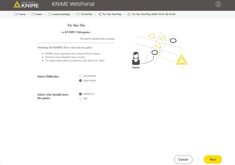
In the Analytics Platform, JavaScript-based nodes for data visualization can build parts of web pages. Encapsulating such JavaScript-based nodes into components allows the construction of dashboards as web pages with fully connected and interactive plots and charts. In particular, we used the Tile View node to display each of the nine sections of the Tic-Tac-Toe board, and show a blank, human, or KNIME icon on each.

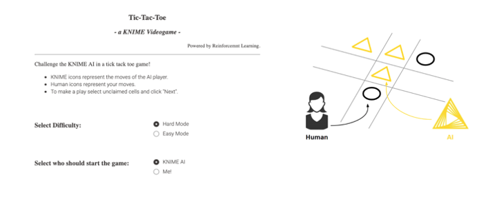
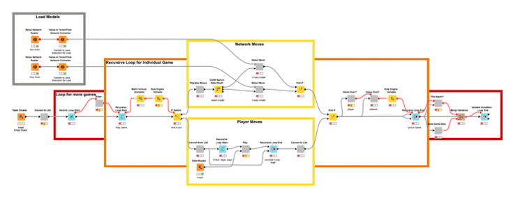
The deployment workflow that allows a human to play (and further train) the agent is shown in Fig. 6. A game session on the resulting web-application is shown in Fig. 7.

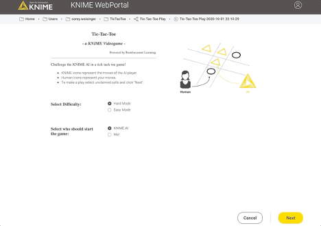
This example of both the learning and playing workflows is available for you to download, play with, and modify on the Hub! I’m curious to see what improvements and use case adaptations you might come with.

Download these workflows from the Hub here:

• Tic-Tac-Toe learning workflow
• Tic-Tac-Toe playing working

Conclusion

In summary, we introduced a few popular use cases for reinforcement learning: drug discovery, traffic regulation, and game AI. On that topic, I encourage you to take to Google and see the many other examples.

We introduced a simple reinforcement learning strategy based on the Markov Decision Process and detailed some key notation that will help you in your own research. Finally, we covered how a simple example can be implemented in my company’s Analytics Platform. 

Originally published on the KNIME blog.