Click to learn more about author Alejandro Correa Bahnsen.
Almost everyone has heard the words “Machine Learning”, but most people don’t fully understand what they mean. Machine Learning isn’t a single formula that is simply applied to a problem. There are many algorithms to choose from, each of which can be used to achieve different goals. This is the first in a series of articles that will introduce Machine Learning algorithms to help you understand how they work, and when to use each one.
What is Machine Learning?
Before we go any further, let’s define exactly what we’re talking about. What is Machine Learning? Machine Learning is about building programs with adaptable parameters that automatically adjust based on the data the programs receive. By adapting to previously seen data, the programs are able to improve their behavior. They also generalize data, meaning that the programs can perform functions on previously unseen datasets.
If that definition brings to mind Artificial Intelligence, then you’re on the right track: Machine Learning is actually a sub-field of Artificial Intelligence. Machine Learning algorithms can be thought of as the building blocks that help computers learn to operate more intelligently.
There are two types of Machine Learning algorithms: supervised and unsupervised. Supervised algorithms use input vectors and target vectors (or expected outputs) as training data, whereas unsupervised algorithms only use input vectors. Unsupervised algorithms use a process called clustering to identify the target vectors. This involves creating groups and subgroups within the data.
As an example, imagine that you are teaching a child to identify different types of vegetables. Supervised learning would involve presenting the child with the vegetables and saying, “This is a carrot. These are peas. This is broccoli.” Unsupervised learning would involve presenting the vegetables without giving their names, and having the child classify the vegetables: The carrot is orange, and the peas and broccoli are green. The child would then create a subcategory to distinguish between the green vegetables. The peas are green and small, and the broccoli is green and big.
Understanding Decision Trees
The first algorithm I’m going to introduce is the decision tree. It’s an older algorithm that is not widely used today, but it still remains important as a foundation for learning the more advanced algorithms that we’ll present.
A decision tree is a supervised predictive model. It can learn to predict discrete or continuous outputs by answering questions based on the values of the inputs it receives.
Let’s look at an example using a real-world dataset: Major League Baseball (MLB) player data from 1986-1987. We’re going to determine a professional player’s salary based on the number of years he’s played in the major leagues and the number of hits he had in the previous year.
The graph below illustrates our training data. The colored dots represent an individual player’s salary: blue/green dots represent low salaries, and red/yellow represent high ones.
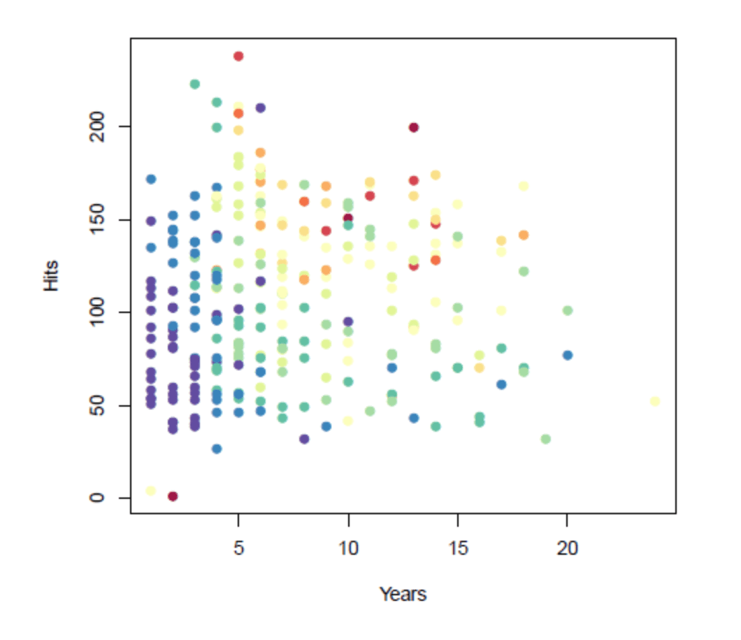
Decision trees use different attributes to repeatedly split the data into subsets until the subsets are pure, meaning that they all share the same target value. In this case, we will segment the space into regions and use the mean salary in each region as the predicted salary for future players. The objective is to maximize the similarity within a region, while minimizing the similarity between regions.
A computer created the following regions:
R1 –less than five years of experience/mean salary of $166,000
R2 –five or more years of experience/less than 118 hits/mean salary of $403,000
R3 –five or more years of experience/118 hits or more/mean salary of $846,000
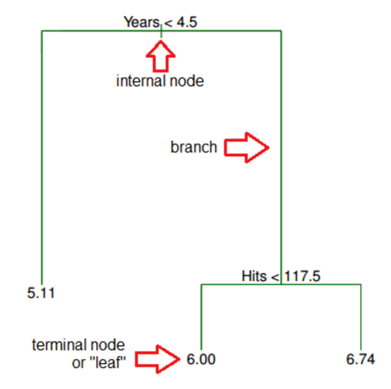
These regions are then used to make predictions on out-of-sample data. Note: there are only three predictions. Here is the equivalent regression tree:
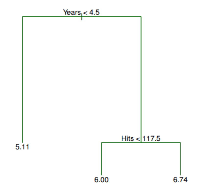
The first split is Years < 4.5, so it goes at the top of the tree. When a splitting rule is true, follow the left branch. When it is false, follow the right branch. The mean salary for players in the left branch is $166,000, thus you label it with that value. (The salary is divided by 1,000 and log-transformed to 5.11.) For players in the right branch, there is a further split on Hits < 117.5. This further divides the players into two more salary regions: $403,000 (transformed to 6.00) and $846,000 (transformed to 6.74).
From this tree, we can deduce the following:
- The number of years a MLB player has played is the most important factor determining his salary, with a lower number of years corresponding to a lower salary.
- For MLB players with a lower number of years, hits are not an important factor in determining salary.
- For MLB players who have played for a higher number of years, hits are an important factor in determining salary, with a greater number of hits corresponding to a higher salary.
Quantifying the Pureness of a Subset
In a decision tree, any attribute can be used to split data, though the algorithm chooses the attribute and condition based on the purity of the resulting subsets. The pureness of a subset is determined by the certainty of the target values within a subset.
To measure the pureness of a subset, we must provide a quantitative measure so that the decision tree algorithm can objectively choose the best attribute and condition to split on. There are a variety of ways to measure uncertainty in a set of values, but for our purposes we’ll use Entropy (represented by H):
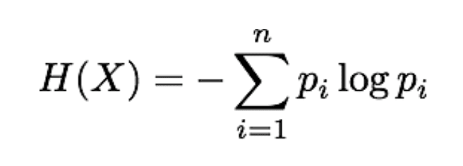
X – the resulting split
n – the number of different target values in the subset
pi – the proportion of the ith target value in the subset
Once an attribute and condition are chosen, you can measure the impurity of the subsets. To do so, we must aggregate the impurity of all subsets into one measure. This is done using the Information Gain Measure, which measures the expected decrease in impurity after a split. The formula for Information Gain is as follows:
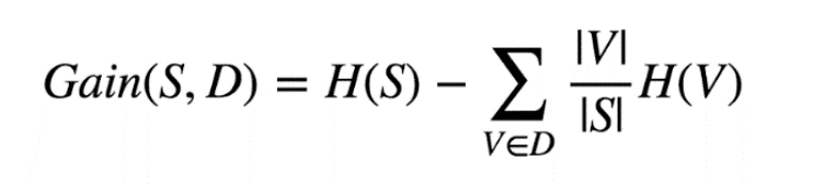
S – the subset before splitting
D – the possible outcome of the splitting using a given attribute and condition
V – assumes that all values D can be measured one by one
The parallel lines on V and S denote the size of the set
Put more simply, the gain calculates the difference in entropy before and after the split.
Summary
Decision trees have a number of advantages and disadvantages that should be considered when deciding whether they are appropriate for a given use case. Advantages include the following:
- Can be used for regression or classification
- Can be displayed graphically
- Highly interpretable
- Can be specified as a series of rules
- More closely approximates human decision-making than other ML algorithms
- Fast prediction
- Features don’t need scaling
- Automatically learns feature interactions
- Tends to ignore irrelevant features
- Non-parametric and therefor will outperform linear models if the relationship between features and response is highly non-linear
The disadvantages of decision trees include the following:
- Performance doesn’t generally compete with the best supervised learning methods
- Can easily overfit the training data, and thus require tuning
- Small variations in the data can result in a completely different tree
- Recursive binary splitting makes “locally optimal” decisions that may not result in a globally optimal tree
- Doesn’t tend to work well with highly unbalanced classes
- Doesn’t tend to work well with very small datasets
Photo Credits: Alejandro Correa Bahnsen